Wednesday 28 October 2015

OTSU thresholding

What is Image Thresholding?

Thresholding is a image processing method used to convert a grey scale image (value of pixels ranging from 0-255) into binary image (value of pixels can have only 2 values: 0 or 1). Thresholding techniques are mainly used in segmentation  The simplest thresholding methods replace each pixel in an image with a black pixel if the pixel intensity is less than some fixed constant T, else it is replace with a white pixel.
If I (i,j) is the intensity at point (i,j) in an image, then:
I(i,j) = 0 if I(i,j)<T
else I(i,j) = 1  
where T is some threshold value.

There are two basic types of thresholding methods:
Static image thresholding
Dynamic image thresholding

More simple and straight forward approach is taken in static thresholding. A pre-determined threshold value is used for segmentation in static image thresholding. It is effective when the background conditions in which image is captured are well known and they do not change. But, if they change, will the threshold value be effective in image segmentation?
Well as you must have correctly recognised, it wont. For instance, the static or pre-determined threshold value wont be effective for handling illumination changes.

What do you do in such conditions? We have dynamic thresholding methods to rescue. They are not effected by such changes. Now, there are various dynamic thresholding techniques, of which the one I found very interesting is OTSU thresholding. I will try explaining the algorithm in detail in this post. 

OTSU Thresholding:

This method is named after its inventor Nobuyuki Otsu and is one of the many binarization algorithm. The post here will describe how the algorithm works and C++ implementation of algorithm. OpenCV has in-built implementation of OTSU thresholding technique which can be used. 

The algorithm assumes that the image contains two classes of pixels following bi-modal histogram (foreground pixels and background pixels), it then calculates the optimum threshold separating the two classes so that their combined spread (intra-class variance) is minimal, or equivalently (because the sum of pairwise squared distances is constant), so that their inter-class variance is maximal. Consequently, Otsu's method is roughly a one-dimensional, discrete analog of Fisher's Discriminant Analysis. Otsu's thresholding method involves iterating through all the possible threshold values and calculating a measure of spread for the pixel levels each side of the threshold, i.e. the pixels that either fall in foreground or background. The aim is to find the threshold value where the sum of foreground and background spreads is at its minimum.


Algorithm steps:


  1. Compute histogram and probabilities of each intensity level.
  2. Set up initial class probability and initial class means.
  3. Step through all possible thresholds maximum intensity.
  4. Update qi and μi.
  5. Compute between class variance.
  6. Desired threshold corresponds to the maximum value of between class variance.

Example: 

The example below is taken from this page. The algorithm will be demonstrated using the simple 6x6 image shown below. The histogram for the image is shown next to it. To simplify the explanation, only 6 greyscale levels are used.
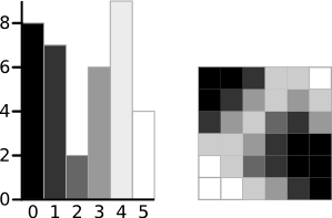
A 6-level greyscale image and its histogram
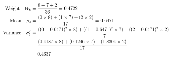
The calculations for finding the foreground and background variances (the measure of spread) for a single threshold are now shown. In this case the threshold value is 3.
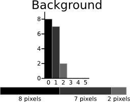
Background levels
Otsu threshold calculation of background
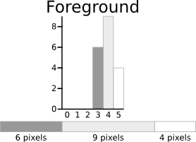
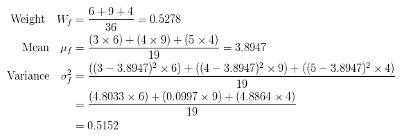
Foreground levels
Otsu threshold calculation of foreground
The next step is to calculate the 'Within-Class Variance'. This is simply the sum of the two variances multiplied by their associated weights.
Otsu threshold calculation of sum of Weighted variances
This final value is the 'sum of weighted variances' for the threshold value 3. This same calculation needs to be performed for all the possible threshold values 0 to 5. The table below shows the results for these calculations. The highlighted column shows the values for the threshold calculated above.


It can be seen that for the threshold equal to 3, as well as being used for the example, also has the lowest sum of weighted variances. Therefore, this is the final selected threshold. All pixels with a level less than 3 are background, all those with a level equal to or greater than 3 are foreground. As the images in the table show, this threshold works well.
Result of Otsu's Method
This approach for calculating Otsu's threshold is useful for explaining the theory, but it is computationally intensive, especially if you have a full 8-bit greyscale. The next section shows a faster method of performing the calculations which is much more appropriate for implementations.

A Faster Approach

By a bit of manipulation, you can calculate what is called the between class variance, which is far quicker to calculate. Luckily, the threshold with the maximum between class variance also has the minimum within class variance. So it can also be used for finding the best threshold and therefore due to being simpler is a much better approach to use.
Simplification of Otsu's threshold calculation


Implementation:

The OpenCV / C++ implementation of OTSU thresholding can be downloaded from here.
OpenCV also a built-in function from thresholding using OTSU method, which can be used as:

    cv::threshold(im_gray, img_bw, 0, 255, CV_THRESH_BINARY | CV_THRESH_OTSU);
    
    where 'im_gray' is the gray image for which thresholding value has to be calculated. 'img_bw' is the black and white image obtained after using OTSU thresholding method on gray image. 

    Advantages
    • Speed: Because Otsu threshold operates on histograms (which are integer or float arrays of length 256), it’s quite fast.
    • Ease of coding: Approximately 80 lines of very easy stuff.


    Disadvantages
    • Assumption of uniform illumination.
    • Histogram should be bimodal (hence the image).
    • It doesn’t use any object structure or spatial coherence.
    • The non-local version assumes uniform statistics.

    Monday 12 October 2015

    Video into JPEG frames

    What is a video? A video is collection of frames, displayed at such a rate that we see a continuous and very smooth motion and we do not perceive the individual frames. It works on the concept of persistence of vision. Generally, a video has upto 24fps to 30 fps (frames per second) i.e 24 to 30 frames are displayed within one second.

    There are various applications where you want to extract individual frames and using them for various computer vision applications like optical flow etc. Having individual frames and saving them as jpeg files may not be a difficult task, but it has significant importance. Lets see how simple this task is.


    VideoCapture:

    The class provides C++ API for capturing video from cameras or for reading video files and image sequences. Here is how VideoCapture can be used: 


    The name of the video is given as command line argument. Now the class VideoCapture will access the individual frames of the video one at a time. The imshow function displays the individual frames with certain wait time. Now, the individual frame is saved to the folder 'frames' which you must have created in the directory where the binary code is present.


    Number of frames saved depends on the fps and the duration of the video. The !frame.data checks if the frame extracted has some data and breaks the loop once the last frame of video has been extracted. Now, go to the directory and see the individual frames saved there. Subscribe to regularly get updates in your mail box. Cheers!!

    Tuesday 6 October 2015

    Training your own Object Detector

    Hello people! Hope you all are enjoying the journey of learning computer vision with me. Remember, the OpenCV code we wrote for face detection. We had used the pre-built classifier 'haarcascade_frontalface_alt.xml’. Did you guys think on what this the xml file is? How was it generated? How can you have your xml file which will help you have a model capable of detecting objects of your interest? 
    Here, we will try to answer all of your above questions and at the end you will be in a position to have your own model. 

    Training your model:

    The xml file is cascade trained for object detection as you may have correctly predicted. Now to train a cascade, you will need loads of data i.e images of objects you want your model to be able to recognise. You will also need images which do not contain the object of your interest. The images with the object in them are referred to as ‘Positive images’ and images without the object are called ‘Negative images’. Here, I will be using the database of cars freely available at this lhttp://cogcomp.cs.illinois.edu/Data/Car/


    It has 550 positive , 500 negative and few test images to check the cascade we just trained ourselves. Now that we have the dataset of cars,we will have a model trained which is capable of detecting cars in unknown images. We would now want all the image details be listed with the correct names so that reading those images from folder isn’t a problem. One way is to type down all the names manually in text file and drain your energy doing nothing good. Other option is using a ubuntu inbuilt command. I and all the smart people ( which you are since you are reading this blog :P) will go for second option.
    Open the terminal on your system. Go to folder where the car images are present. For convenience I have the positive and negative image folder saved on desktop. So I will do the following:  


    This will create a info.txt file in the folder with all the image files listed. We would now give it the absolute path so that we can use the details from the desktop directory too.  Same is repeated for negative images.


    Now I have the list of positive and negative images ready. The list of positive images should have one more detail with its name i.e the location where the object of our interest is present. In this case we have the isolated cars in images and all have the same dimension. This simplifies the work for us. You should now have the info.txt as shown below: 


    I will now move the info.txt and neg.txt to Desktop.

    The training of cascade requires the data of object to be present in a ‘vec file’. So we will now have the vec file generated. The command should do the work for you. 

    $opencv_createsamples -info info.txt -num 500 -w 48 -h 24 -vec car.vec 


    The width and height are set to that ratio since the car has greater width and lesser height. Also, the number of samples we use is generally less than the number of actual images we have and so we take 500 in this case. Now create a folder ‘data’ which will contain all the information of training stages and also have the final trained cascade.

    Now run the command 

    $opencv_traincascade -data data -vec car.vec bg neg.txt -numPos 400 -numNeg 500 -numStages 13 -w 48 -h 24 -featureType LBP -maxFalseAlarmRate 0.4 -minHitRate 0.99 -precalcValBufSize 20488 -precalcIdxBufSize 2048


    This command has started the training process for cascade. You will see something like this:


    Depending upon the number of stages we want the cascade to train itself, it will take sometime and the process will complete. This should take good amount of time depending your system configuration. Also, the number of images we took here is quiet less if we want the cascade to be very accurate. And increasing the number of images will definitely add to the time consumption.  You can see something like this:


    Now, you can see the cascade.xml in the data folder. It also has various stage.xml. The stage.xml is the result obtained after it has completed that many stages of training. It may not really seem useful since we already have obtained the final cascade within hardly some significant time. That may not be case always, especially when the dimensions of the object is big and large number of images are used. Now, imagine that the training stops due to some unexpected interruption like power cut or something that sort. How frustrating it would be start the training all over again and wasting the time. This is where the stages.xml come to rescue. The training will resume only from the stage where it last stopped and not from stage 0. 
    Thus, you have now trained the cascade for car detection. You can definitely go ahead with training your object detector! Now its time to check how does the cascade work. So pick up any image from the test data set or whichever image of car you have. The only thing to make sure is that car has the shape similar to the images which were used for training.

    Copy the code given below and keep your fingers crossed.


    Yeah!! The car detector worked. Now start collecting the images of object you would like your model to recognise and start training the cascade. Explaining every steps in details was not possible right now. Do write to me, if you get struck somewhere or have any particular doubts. Subscribe to regularly get updates in your mail box.
    CheERs!!


    Wednesday 30 September 2015

    Hough Transforms

    The Hough transform is a feature extraction technique used in image analysis and computer vision. The purpose of the technique is to find imperfect instances of objects within a certain class of shapes by a voting procedure. The classical Hough transform was developed with the intention of being able to identify straight lines in the image, but later the Hough transform has been extended to identifying positions of arbitrary shapes, most commonly circles or ellipses. This post will involve a bit of math, but just elementary concepts you learned in school.  Also, we'll work with lines only, though the technique can be easily extended to other shapes. 

    Why Hough transform?

    Suppose you have image of straight road. You figure out edge pixels (using the Canny edge detector, the Sobel edge detector, or any other thing). Now you want a geometrical representation of the pole's edge. But right now the "edge" is just a sequence of pixels. You can loop through all pixels, and some how figure out the slope and intercept. But that is one difficult task. Images are never perfect. So you want some mechanism that give more weightage to pixels that are already in a line. This is exactly what the Hough Transform does.  It lets each point on the image "vote". And because of the mathematical properties of the transform, this "voting" allows us to figure out prominent lines in the image. Don’t worry if you like a tail-ender facing a bouncer ball. You should soon be able to face them with ease.!

    The mathematics behind hough transform:

    Convert line to point:

    A lines is a collection of points. And managing a collection of points is tougher than managing a single point. Obviously. So the first thing we learn is how to represent a line as a single point, without losing any information about it.
    This is done through the m-c space.


    As shown in the above picture, every line has two quantities associated with it, the slope and the intercept. With these two numbers, you can describe a line completely.
    So the parameter space, or the mc space was devised. Every line in the xy space is equivalent to a single point in the mc space.

    Convert point to line

    Now onto the next step. Consider a point (say, (xa, ya) )in the xy space. What would its representation in the mc space be?
    For starters, you could guess that infinite lines pass through a point. So, for every line passing through (xa, ya), there would be a point in the mc space.
    And you're correct there, because of the following:
    1. Any line passing through (xa, ya): ya = mxa + c
    2. Rearranging: c = - xam + ya
    3. The above is the equation of a line in the mc space.


    So, a point in the xy space is equivalent to a line in the mc space.


    Now we know conversion of points to line and vice-versa.  Now, if we observe each intersection point, then we can easily see that intersection point of line 1 and line 2 represents the slope and intercept of the line passing through point 1 and point 2. Similary, intersection point of line 3 and line 4 represents the slope and the intercept of the line passing through point 3 and point 4. 


    The interesction point of line 1, line 2 and line 3 represents the slope and the intercept of the line passing through point 1, point 2 and point 3.
    So we can see that the point which is the common interception of more number of lines will represent the slope and intercept of the line passing through more number of points. And similary, if a point has only one passing through line in mc space, it will represent a line which passes through only one edge point. If a large number of lines intersect at same point, we can say that the line in xy space for that point is more dominant line. Thus, we can identify edge points in image which lie on same straight line.

    Hough Space:

    There is a flaw in the method which we just discussed. The value of slope i.e m tends to infinity for the vertical lines. So, we need to have infinite memory to store the ‘mc space’. So we have a work around this which will helps us maintain the concept but won’t have high memory requirements.
    We use polar co-ordinates for this purpose. 
     r = x1cos(Θ)+y1sin(Θ)
    where Θ is the angle that normal from the origin to the line makes with the x-axis and r is the perpendicular distance of the line from the origin.


    Range of parameters:
    1. Θ varies from -90 to +90.
    2. r varies from 0 to the diagonal length of the image.
    With this new representation, we have a new transition from xy plane to Hough plane. A line in the xy space still represents a point in Hough space (pΘ plane here). But a point in xy space represents a sinusoid in r-Θ space.

    Actual implementation:

    We have edge points in the images detected using one of edge detector i.e canny edge detector, sober detector and so on. Now every non-black pixel (i.e pixel which lies on edge ) is represented on hough space. A 2D accumulator is created which accumulates votes of each point represented by each cell of the accumulator. In our case, the accumulator cells form a 2D array. The horizontal axis is for the different θ values and the vertical axis for p values. 


    You choose a sinusoidal and vary Θ to get different r. You take the value of Θ and obtain corresponding value of r and cast a vote in the particular (Θ, r) accumulator cell. By voting, you increase the value of the cell by 1. After voting, you choose another value of Θ and vote in corresonding accumulator cell by Θ and r. Continue doing this from Θ=-90 to Θ=+90. And for every such calculation, you add vote in the accumulator.


    Depending on the number of votes at each cell in accumulator, we will obtain the line which will be the best fit for a certain set of points. More the number of votes at a particular cell (i.e. r and Θ), more number of points lie on that line. In the hough space diagram, the bright spots denote more number of points voted for that spot. Thus, we can have straight lines in the image detected using hough transform. Now, get your fingers ready and start implementing it on your machine!!  
    Subscribe to regularly get updates in your mail box.

    Tuesday 29 September 2015

    Machine learning: Lets dig into it!!

    Machine learning is the fascinating term for most of us. I am sure that even you are among one of those curious beings on this planet, who wants answer to few of the following questions: 

    1) Why is topic on machine learning here? 
    2) What exactly is Machine Learning all about?
    3) How do you use it in real world problems?
    4) Which all problems can be solved using Machine Learning?
    5) I am aware that it requires lots of data. What exactly does this data mean? How much data is necessary?
    6) How accurate will machine learning algorithm prove?
    7) Is it worth all the recognition it has received in the recent years?
    Give your curious wings some rest and lets walk slowly through all the content calmly. I will try to cover basics of machine learning in separate topics. I will also get into details of few algorithms that are widely used today. So lets get started ! 


    What is Machine Learning?


    Machine learning is a type of artificial intelligence (AI) that provides computers with the ability to learn without being explicitly programmed. Machine learning focuses on the development of computer programs that can teach themselves to grow and change when exposed to new data. It evolved from the study of pattern recognition and computational learning theory in artificial intelligence. Machine learning explores the study and construction of algorithms that can learn from the data sets provided and make predictions on new data. Such algorithms operate by building a model from example inputs in order to make data-driven predictions or decisions, rather than following strictly static program instructions.  
    Examples:
    1) Machine learning can help you predict what will the temperature in city X studying the pattern of temperature for last few days in that city.
    2) Machine learning can help the us detect whether a tumour is malignant or not.
    3) Machine learning can help us predict whether a particular product will be bought by customer depending upon the previous purchase patterns.

    Machine Learning problems can be classified into following categories:
    1) Supervised Machine Learning
    2) Unsupervised Machine Learning
    3) Semi-supervised Machine Learning
    4) Reinforcement Machine Learning
    5) Deep Learning

    Today, a lot of computer vision techniques have been integrated with machine learning, improving the results observed. I myself have been using machine learning with computer vision algorithms. Here, we will be dwelling deeper into supervised and unsupervised form of learning as and when the necessary concepts need to be explained. 

    1) Supervised Machine Learning:

    In a supervised learning algorithm, the data is a set of training examples with the associated “correct answers”. Supervised learning is a type of machine learning algorithm that uses a known dataset (called the training dataset) to make predictions. The training dataset includes input data and response values. From it, the supervised learning algorithm seeks to build a model that can make predictions of the response values for a new dataset. A test dataset is often used to validate the model. Using larger training datasets often yield models with higher predictive power that can generalize well for new datasets. An example of this would be learning to predict whether an email is spam if given a million emails, each of which is labeled as “spam” or “not spam”. 

    Examples of Supervised Machine Learning:
    1) Decision tree 
    2) Ensembles (Bagging, Boasting, Random Forest)
    3) Linear Regression 
    4) Artificial Neural Networks
    5) Logistic Regression 
    6) Support Vector Machine

    Now, supervised machine learning can be used to perform two types of tasks:

    • classification.
    • regression.
    Output of task performed with regression model will be a continuous value while output will be a discrete label for task performed using classification model. e.g.: the temperature prediction task for city X would be performed using regression model as the temperature value can take continuous value in a particular climate range. On other hand, predicting whether a given tumour is malignant or not is performed using classification model as it will have definite discrete values as output i.e. yes or no ( in our case). The task of optical character recognition is again a classification problem as the output of the model has to be one of the 26 characters for which it has been trained.


    2) Unsupervised Machine Learning: 

    In an unsupervised learning algorithm, the algorithm can find trends in the data it is given, without looking for some specific “correct answer”.  Unsupervised learning is a type of machine learning algorithm used to draw inferences from datasets consisting of input data without labeled responses. The most common unsupervised learning method is cluster analysis, which is used for exploratory data analysis to find hidden patterns or grouping in data. The clusters are modeled using a measure of similarity which is defined upon metrics such as Euclidean or probabilistic distance. Examples of unsupervised learning algorithms involve clustering (grouping similar data points) or anomaly detection (detecting unusual data points in a data set).

    Common clustering algorithms include:

    • 1) Hierarchical clustering
    • 2) k-Means clustering
    • 3) Gaussian mixture models
    • 4) Self-organizing maps
    • 5) Hidden Markov models

    3) Semi-Supervised Machine Learning:

    As the name suggests, Semi-supervised machine learning falls between unsupervised i.e without any unlabeled data and supervised machine learning i.e completely labeled data. Semi-supervised learning is class of supervised learning tasks which also makes use of unlabeled data. Many researchers have found it to be advantageous to use unlabeled data in conjunction with a small amount of labeled data. The semi-supervised learning technique is used with the goal of reducing the amount of supervision required as compared with supervised learning while improving the unsupervised clustering to meet the expectations of user. 


    4) Reinforcement Learning:

    Reinforcement learning is an area of machine learning inspired by behaviorist psychology, concerned with how software agents ought to take actions in an environment so as to maximize some notion of cumulative reward. The problem, due to its generality, is studied in many other disciplines such as game theory, control theory, operations research, information theory, simulation based optimization, multi-agent systems, swarm intelligence, statistics and generic algorithms. In the operations research and coontrol literature, the field where reinforcement learning methods are studied is called approximate dynamic programming.

    5) Deep learning:

    Deep learning(deep machine learning, or deep structured learning, or hierarchical learning, or sometimes DL) is a branch of machine learning based on a set of  algorithms that attempt to model high-level abstractions in data by using model architectures, with complex structures or otherwise, composed of multiple non-linear transformations. Deep learning is part of a broader family of machine learning methods based on learning representations of data. An observation (e.g., an image) can be represented in many ways such as a vector of intensity values per pixel, or in a more abstract way as a set of edges, regions of particular shape, etc. Some representations make it easier to learn tasks (e.g., face recognition or facial expression recognition) from examples. One of the promises of deep learning is replacing handcrafted features with efficient algorithms for unsupervised or semi-supervised feature learning and hierarchical feature extraction.


    We will start getting into details of many of the supervised and unsupervised machine learning algorithms as  mentioned above. I would also highly recommend everyone to take up the machine learning course by Andrew Ng at Coursera. It is one of finest online video lecture course on Machine learning!


    Friday 18 September 2015

    Installing OpenCV for MAC!

    After instructions guide for installing OpenCV on Ubuntu and installing OpenCV for Windows, here is the guide to install OpenCV on Mac. I have been using OpenCV on ubuntu 14.10 for three years now. However, installing OpenCV on Mac was real pain. No appropriate tutorials added to the pain.!! So, finally here is a tutorial which will try to help you out setting up OpenCV on Mac and ease out your help to some extent.


    Prerequisites

    • Make sure you have git command line tool installed on your machine.
    • Make sure Macports is installed on your machine. If not, you can get it here.Install it before you proceed.
    • If you don’t have cmake, run the following command to install it (this command uses Macports): 
    •  $ sudo port install cmake

    Downloading OpenCV

    We are now ready to install OpenCV. Download the latest version of OpenCV from here. Make sure you download the version for your platform (Mac, Windows, etc). You will get a directory named opencv-2.x.x, depending on the latest version number.
    If you don’t want to worry about downloading every time a new version is released, you can download the OpenCV git repo. This way, you can easily maintain and update your OpenCV version with a simple command. Open the terminal, go to a convenient location and download the OpenCV source code using the following command:

    $ git clone git://code.opencv.org/opencv.git
    It will create a directory called “opencv” and download all the files here. When you want to update to a new version, just go to this folder and type the following command:

    $ git pull
    This will update your repo to the latest version.


    Installing OpenCV

    Now that we have the source code for OpenCV, we need to build it. Run the following commands:

    $ cd opencv
    $ mkdir build
    $ cd build
    $ cmake -G "Unix Makefiles" ../
    $ make -j8
    We need to place the libraries in the correct locations so that they are accessible. Run the following command:

    $ sudo make install
    This will install everything in the /usr/local/ directory. That’s it! OpenCV is now installed on your machine.


    OpenCV with Xcode

    Now that we have installed OpenCV, we are ready to use it in our C/C++ code. Xcode is the most popular IDE on Mac OS X, so we would naturally want to see how to use OpenCV on Xcode. I have outlined the procedure below:
    1. Open Xcode
    2. Select Xcode -> New -> Project.
    3. A new window will pop up. On the left sidebar, under “OS X”, select “Application” and choose “Command Line Utility”. Click “Next”
    4. In the next window, give a name for the project and make sure the “Type” field at the bottom is set to C++. Click “Next”
    5. In the left sidebar, you should be able to see your project name next to a small Xcode icon. Double click on the project. This should open the Build Settings tab (located on the top of the new window).
    6. In the “Architectures” section, make sure it is set to “Native architecture of the build machine”.
    7. Scroll down to the “Search Paths” section and set “Header Search Paths” to: /usr/local/include. You can do this by double-clicking on the blank space right next to “Header Search Paths” and clicking on the “+” symbol at the bottom left. After you add it, make sure you select “recursive” located on the end of the same row.
    8. Close this window.
    9. In the left sidebar, you should be able to see your project name with a folder icon next to it. If you expand it, you will see main.cpp. Now right click on this project and select “New group”. Name it “OpenCV Libraries”.
    10. Right click on “OpeCV Libraries” and select Add Files to “Project” … (the word “Project” would have been replaced with your project name)
    11. Press the “/” key to get the “Go to” folder prompt. Enter the following path: /usr/local/lib
    12. Select all the files whose names are of the form libopencv_*.dylib.
      Note: Although you don’t have to worry about this, it’s better to know anyway. There will be aliases in that file list as well. So before selecting a file, look at the file icon. If there’s an arrow on the icon, it means that this file is an alias. You don’t have to add these files, since they are just aliases (and not real files).
    13. Click “Add” and you are done!
    Go to main.cpp and write a simple piece of OpenCV code. Check if it runs. If you see an error, read on.


    Running OpenCV Code From Command Line

    This is the last sure shot way of running OpenCV code, but you will miss out on the niceness of an IDE. You can use cmake to build and run OpenCV code. Open the Finder and create a folder for your project. Place your .cpp file there. Create a file called “CMakeLists.txt” and place the following lines in that file:

    project(PROJECT_NAME)
    cmake_minimum_required(VERSION 2.6 FATAL_ERROR)
    
    find_package(OpenCV REQUIRED)
    
    # Project Executable
    add_executable (filename filename.cpp)
    target_link_libraries(filename ${OpenCV_LIBS})
    In the above lines, replace “PROJECT_NAME” with your project name and replace filename by your source code file name. For example, if your project name is “Image Display” and your filename is “display.cpp”, then the contents of CMakeLists.txt should be:


    project(IMAGE_DISPLAY)
    cmake_minimum_required(VERSION 2.6 FATAL_ERROR)
    
    find_package(OpenCV REQUIRED)
    
    # Project Executable
    add_executable (display display.cpp )
    target_link_libraries(display ${OpenCV_LIBS})
    Once you create this file, run the following commands in the same directory:
    $ cmake .
    $ make
    You should now be able to see the executable with the same name as the your .cpp file. Now open the terminal and just type the following to run the code:

    $ display
    If you have any command line arguments that you are taking in your .cpp file, give them here:

    $ tracker arg1 arg2
    And there you go! You are all set to do some OpenCV coding!! Subscribe to regularly get updates in your mail box.

    Wednesday 2 September 2015

    Installing OpenCV-2.4.11 on Windows 7

    After having written a detailed guide on Installing OpenCV-2.4.11 for Ubuntu, I got few emails requesting me to have a guide for installing OpenCV libraries on Windows. So, here is a guide for Windows users. Here in this tutorial I am going to show how to configure Visual Studio 2010 to use OpenCV 2.4.11 in your computer vision projects. Also, I am going to write a couple of lines of code to show that OpenCV has correctly been installed. And yes, you can definitely expect a guide for Mac soon.!


    We have two options for installing opencv-2.4.11 to work with the Visual Studio on Windows:
    1) Installation by using the Pre-built libraries. 
    2) Installation by Making your own Libraries from Source files.


    While the first one is easier to complete, it only works if you are coding with the latest Microsoft Visual Studio IDE and doesn’t take advantage of the most advanced technologies we integrate into our library. Here, we will dig deeper into using the pre-built libraries for the simplicity of installation that it offers. 

    Downloading and Installing OpenCV-2.4.11 for Windows:

    In this tutorial, I will assume that you have successfully installed Visual Studio on your Windows computer. 
    2) Now go to the folder where you have the downloaded the executable file and choose to ‘Run as Administrator’.
    3) The executable file is essentially an archive of files with an extractor built in. It will ask you to select the location where you would like it to extract all its contents. 


    Select: C:\Program Files\ as the path and click Extract. It will create a folder called OpenCV2.4.11 with the path: C:\Program Files\OpenCV2.4.11.

    Manually Changing the System Path to Include the Bin File:

    1) To access the system path in Vista go to Control Panel\System and Security\System and on the left hand side select Advanced system settings this should bring up the Systems Properties dialogue.  Click on the Advanced tab and then the Environment Variables button.


    2) This will bring up the Environment Variables dialogue.  In the System Variables box select Path and then Edit


    3)When modifying the path know that it is sensitive to all characters including spaces.  To add the new bin, type a semicolon directly after the text that is there without adding in a space.  Next add the path to the bin file.  The path is the same as where you chose to install OpenCV back in step 3 of Downloading and Installing OpenCVsection plus \bin. 


    For 64 bit Windows, add the following to the system path:
    ;C:\Program Files\OpenCV2.4.11\build\bin\;C:\Program Files\OpenCV2.3\build\x64\vc10\bin\


    Make sure to restart your computer so the changes can take effect.

    Configuring Visual Studio


    1) Click Project Properties to access the properties dialog


    2) In the left box click on Configuration Properties and on the top right click onConfiguration      Manager


    3) In the Configuration Manager dialog box that opens up, under Active Solution Platform combo box select New.


    4) In the New Solution Platform dialog box that opens up, under Type or select the new platform, select x64, copy settings from Win32 and make sure that Create new project platforms is selected. Click OK.


    5) You will notice that the in the Configuration Manager dialog box x64 platform has now been selected. Click Close.


    6) In the left box choose Configuration Properties C++ General


    7) In the right box, next to Additional Include Directories type the following text:C:\Program Files\OpenCV2.3\build\include;C:\Program Files\OpenCV2.3\build\include\opencv;


    IMPORTANT: note that all these paths assume that you installed in the default location, if you installed in a different location; for example Program Files (x86) instead of Program Files, make sure you change these paths to reflect that.

    8)  Next in the felt box choose Configuration Properties Linker Input


    9) In the right box, next to Additional Dependencies type the following text:
    "C:\Program Files\OpenCV2.4.11\build\x64\vc10\lib\opencv_core24110d.lib";
    "C:\Program Files\OpenCV2.4.11\build\x64\vc10\lib\opencv_highgui2411d.lib";
    "C:\Program Files\OpenCV2.4.11\build\x64\vc10\lib\opencv_video2411d.lib";
    "C:\Program Files\OpenCV2.4.11\build\x64\vc10\lib\opencv_ml2411d.lib";
    "C:\Program Files\OpenCV2.4.11\build\x64\vc10\lib\opencv_legacy2411d.lib";
    "C:\Program Files\OpenCV2.4.11\build\x64\vc10\lib\opencv_imgproc2411d.lib";

    IMPORTANT: note that all these paths assume that you installed in the default location, if you installed in a different location; for example Program Files (x86) instead of Program Files, make sure you change these paths to reflect that.

    10) Click Apply then OK


    Hello OpenCV

    OK. Now we are (almost) ready to write our first lines of code. Switch to "Solution Explorer" by clicking the tab below. Right click on "Source Files", select "Add" -> "New Item...". Select "C++ File" from the menu and type "main" as name.


    Insert the following lines into the main.cpp and run the code (press F5).

    #include "opencv2/highgui/highgui.hpp"
    #include <iostream>

    using namespace cv;
    using namespace std;

    int main( int argc, const char** argv )
    {
      Mat img = imread("lena.png", CV_LOAD_IMAGE_UNCHANGED); //read the image data in the file "lena.png" and store it in 'img'

    if (img.empty()) //check whether the image is loaded or not
    {
    cout << "Error : Image cannot be loaded..!!" << endl;
    return -1;
    }

    namedWindow("image", CV_WINDOW_AUTOSIZE); //create a window with name "MyWindow"
    imshow("image", img); //display the image which is stored in the 'img' in "MyWindow" window


    waitKey(0); //wait infinite time for a keypress
         destroyWindow("MyWindow"); //destroy the window with the name, "MyWindow"
    return 0;
    }


    NOTE: You need to add the image to the project folder else you need to provide the absolute path to image. The code above will load the image and display it as shown in output above. You can easily use any image of your choice, just make sure you give the absolute path to image with correct image name.


    Tips / Common Errors:
    1) Check if you are using the right lib files: Do not mix 32 bit (x86) and 64 bit (x64) directories.

    2) If you are using the pre-build OpenCV package, add the right include directory to your Visual Studio project. The include directory is NOT <path to your unzipped OpenCV directory>\opencv\includes. Use <path to your unzipped OpenCV directory>\opencv\build\includes instead!

    3) Application start fails: Check if the system can locate the OpenCV DLLs (these either have to reside on a system path or in the same directory as the application).

    4) Additionally, you might see the error message that “tbb_debug.dll” is missing when starting your application. The “Intel® Threading Building Blocks” needs to be installed (partly) as well. Therefore, download the latest stable release for your OS at http://threadingbuildingblocks.org/download.php. If you unzip the files, you might either install the whole package or at least copy the tbb_debug.dll (check OS, 32 oder 64 bit, VS version) to the same directory as your application.

    Hope that this guide helps you get started with OpenCV on Windows. Comments and Feedback are most welcomed!!