OTSU thresholding

What is Image Thresholding?

Thresholding is a image processing method used to convert a grey scale image (value of pixels ranging from 0-255) into binary image (value of pixels can have only 2 values: 0 or 1). Thresholding techniques are mainly used in segmentation  The simplest thresholding methods replace each pixel in an image with a black pixel if the pixel intensity is less than some fixed constant T, else it is replace with a white pixel.

If I (i,j) is the intensity at point (i,j) in an image, then:

I(i,j) = 0 if I(i,j)<T

else I(i,j) = 1  

where T is some threshold value.

There are two basic types of thresholding methods:

Static image thresholding

Dynamic image thresholding

More simple and straight forward approach is taken in static thresholding. A pre-determined threshold value is used for segmentation in static image thresholding. It is effective when the background conditions in which image is captured are well known and they do not change. But, if they change, will the threshold value be effective in image segmentation?
Well as you must have correctly recognised, it wont. For instance, the static or pre-determined threshold value wont be effective for handling illumination changes.

What do you do in such conditions? We have dynamic thresholding methods to rescue. They are not effected by such changes. Now, there are various dynamic thresholding techniques, of which the one I found very interesting is OTSU thresholding. I will try explaining the algorithm in detail in this post. 

OTSU Thresholding:

This method is named after its inventor Nobuyuki Otsu and is one of the many binarization algorithm. The post here will describe how the algorithm works and C++ implementation of algorithm. OpenCV has in-built implementation of OTSU thresholding technique which can be used. 

The algorithm assumes that the image contains two classes of pixels following bi-modal histogram (foreground pixels and background pixels), it then calculates the optimum threshold separating the two classes so that their combined spread (intra-class variance) is minimal, or equivalently (because the sum of pairwise squared distances is constant), so that their inter-class variance is maximal. Consequently, Otsu's method is roughly a one-dimensional, discrete analog of Fisher's Discriminant Analysis. Otsu's thresholding method involves iterating through all the possible threshold values and calculating a measure of spread for the pixel levels each side of the threshold, i.e. the pixels that either fall in foreground or background. The aim is to find the threshold value where the sum of foreground and background spreads is at its minimum.

Algorithm steps:

1. Compute histogram and probabilities of each intensity level.
2. Set up initial class probability and initial class means.
3. Step through all possible thresholds maximum intensity.
4. Update qi and μi.
5. Compute between class variance.
6. Desired threshold corresponds to the maximum value of between class variance.

Example: 

The example below is taken from this page. The algorithm will be demonstrated using the simple 6x6 image shown below. The histogram for the image is shown next to it. To simplify the explanation, only 6 greyscale levels are used.

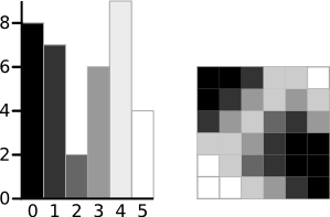
A 6-level greyscale image and its histogram

The calculations for finding the foreground and background variances (the measure of spread) for a single threshold are now shown. In this case the threshold value is 3.

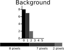
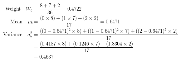
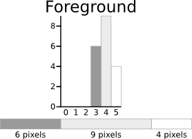
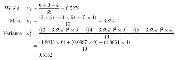
The next step is to calculate the 'Within-Class Variance'. This is simply the sum of the two variances multiplied by their associated weights.

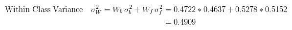
This final value is the 'sum of weighted variances' for the threshold value 3. This same calculation needs to be performed for all the possible threshold values 0 to 5. The table below shows the results for these calculations. The highlighted column shows the values for the threshold calculated above.

It can be seen that for the threshold equal to 3, as well as being used for the example, also has the lowest sum of weighted variances. Therefore, this is the final selected threshold. All pixels with a level less than 3 are background, all those with a level equal to or greater than 3 are foreground. As the images in the table show, this threshold works well.

Result of Otsu's Method

This approach for calculating Otsu's threshold is useful for explaining the theory, but it is computationally intensive, especially if you have a full 8-bit greyscale. The next section shows a faster method of performing the calculations which is much more appropriate for implementations.

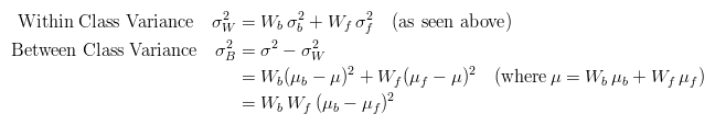
A Faster Approach

By a bit of manipulation, you can calculate what is called the between class variance, which is far quicker to calculate. Luckily, the threshold with the maximum between class variance also has the minimum within class variance. So it can also be used for finding the best threshold and therefore due to being simpler is a much better approach to use.

Implementation:

The OpenCV / C++ implementation of OTSU thresholding can be downloaded from here.

OpenCV also a built-in function from thresholding using OTSU method, which can be used as:

cv::threshold(im_gray, img_bw, 0, 255, CV_THRESH_BINARY | CV_THRESH_OTSU);

where 'im_gray' is the gray image for which thresholding value has to be calculated. 'img_bw' is the black and white image obtained after using OTSU thresholding method on gray image. 

Advantages

• Speed: Because Otsu threshold operates on histograms (which are integer or float arrays of length 256), it’s quite fast.
• Ease of coding: Approximately 80 lines of very easy stuff.

Disadvantages

• Assumption of uniform illumination.
• Histogram should be bimodal (hence the image).
• It doesn’t use any object structure or spatial coherence.
• The non-local version assumes uniform statistics.

Video into JPEG frames

What is a video? A video is collection of frames, displayed at such a rate that we see a continuous and very smooth motion and we do not perceive the individual frames. It works on the concept of persistence of vision. Generally, a video has upto 24fps to 30 fps (frames per second) i.e 24 to 30 frames are displayed within one second.

There are various applications where you want to extract individual frames and using them for various computer vision applications like optical flow etc. Having individual frames and saving them as jpeg files may not be a difficult task, but it has significant importance. Lets see how simple this task is.

VideoCapture:

The class provides C++ API for capturing video from cameras or for reading video files and image sequences. Here is how VideoCapture can be used: 

The name of the video is given as command line argument. Now the class VideoCapture will access the individual frames of the video one at a time. The imshow function displays the individual frames with certain wait time. Now, the individual frame is saved to the folder 'frames' which you must have created in the directory where the binary code is present.

Number of frames saved depends on the fps and the duration of the video. The !frame.data checks if the frame extracted has some data and breaks the loop once the last frame of video has been extracted. Now, go to the directory and see the individual frames saved there. Subscribe to regularly get updates in your mail box. Cheers!!

Training your own Object Detector

Hello people! Hope you all are enjoying the journey of learning computer vision with me. Remember, the OpenCV code we wrote for face detection. We had used the pre-built classifier 'haarcascade_frontalface_alt.xml’. Did you guys think on what this the xml file is? How was it generated? How can you have your xml file which will help you have a model capable of detecting objects of your interest? 

Here, we will try to answer all of your above questions and at the end you will be in a position to have your own model. 

Training your model:

The xml file is cascade trained for object detection as you may have correctly predicted. Now to train a cascade, you will need loads of data i.e images of objects you want your model to be able to recognise. You will also need images which do not contain the object of your interest. The images with the object in them are referred to as ‘Positive images’ and images without the object are called ‘Negative images’. Here, I will be using the database of cars freely available at this lhttp://cogcomp.cs.illinois.edu/Data/Car/. 

It has 550 positive , 500 negative and few test images to check the cascade we just trained ourselves. Now that we have the dataset of cars,we will have a model trained which is capable of detecting cars in unknown images. We would now want all the image details be listed with the correct names so that reading those images from folder isn’t a problem. One way is to type down all the names manually in text file and drain your energy doing nothing good. Other option is using a ubuntu inbuilt command. I and all the smart people ( which you are since you are reading this blog :P) will go for second option.

Open the terminal on your system. Go to folder where the car images are present. For convenience I have the positive and negative image folder saved on desktop. So I will do the following:  

This will create a info.txt file in the folder with all the image files listed. We would now give it the absolute path so that we can use the details from the desktop directory too.  Same is repeated for negative images.

Now I have the list of positive and negative images ready. The list of positive images should have one more detail with its name i.e the location where the object of our interest is present. In this case we have the isolated cars in images and all have the same dimension. This simplifies the work for us. You should now have the info.txt as shown below: 

I will now move the info.txt and neg.txt to Desktop.

The training of cascade requires the data of object to be present in a ‘vec file’. So we will now have the vec file generated. The command should do the work for you. 

$opencv_createsamples -info info.txt -num 500 -w 48 -h 24 -vec car.vec 

The width and height are set to that ratio since the car has greater width and lesser height. Also, the number of samples we use is generally less than the number of actual images we have and so we take 500 in this case. Now create a folder ‘data’ which will contain all the information of training stages and also have the final trained cascade.

Now run the command 

$opencv_traincascade -data data -vec car.vec bg neg.txt -numPos 400 -numNeg 500 -numStages 13 -w 48 -h 24 -featureType LBP -maxFalseAlarmRate 0.4 -minHitRate 0.99 -precalcValBufSize 20488 -precalcIdxBufSize 2048

This command has started the training process for cascade. You will see something like this:

Depending upon the number of stages we want the cascade to train itself, it will take sometime and the process will complete. This should take good amount of time depending your system configuration. Also, the number of images we took here is quiet less if we want the cascade to be very accurate. And increasing the number of images will definitely add to the time consumption.  You can see something like this:

Now, you can see the cascade.xml in the data folder. It also has various stage.xml. The stage.xml is the result obtained after it has completed that many stages of training. It may not really seem useful since we already have obtained the final cascade within hardly some significant time. That may not be case always, especially when the dimensions of the object is big and large number of images are used. Now, imagine that the training stops due to some unexpected interruption like power cut or something that sort. How frustrating it would be start the training all over again and wasting the time. This is where the stages.xml come to rescue. The training will resume only from the stage where it last stopped and not from stage 0. 

Thus, you have now trained the cascade for car detection. You can definitely go ahead with training your object detector! Now its time to check how does the cascade work. So pick up any image from the test data set or whichever image of car you have. The only thing to make sure is that car has the shape similar to the images which were used for training.

Copy the code given below and keep your fingers crossed.

Yeah!! The car detector worked. Now start collecting the images of object you would like your model to recognise and start training the cascade. Explaining every steps in details was not possible right now. Do write to me, if you get struck somewhere or have any particular doubts. Subscribe to regularly get updates in your mail box.

CheERs!!